QUBOs: Getting Started#
Solve QUBOs to Global Optimality with Quantagonia’s HybridSolver
Setup
Using the Quantagonia API client is as easy as pip-installing it and setting your API key.
!pip install hybridsolver
import hybridsolver
API_KEY="Your-API-KEY" # if you don't have one, head over to https://platform.quantagonia.com/ (free account available)
We also setup some standard packages.
# import packages
import networkx as nx
import matplotlib.pyplot as plt
Example: MaxCut as QUBO
In order to demonstrate the QUBO capabilities of Quantagonia’s HybridSolver, we consider the classic MaxCut problem. MaxCut seeks to partition a set of nodes into two complementary subsets such that the number of edges between these two node sets is as large as possible. MaxCut has many applications, e.g., in statistical physics or VLSI design and circuit layout design. In particular, MaxCut is equivalent to minimizing the Hamiltonian of a spin glass model.
Build a Random Graph
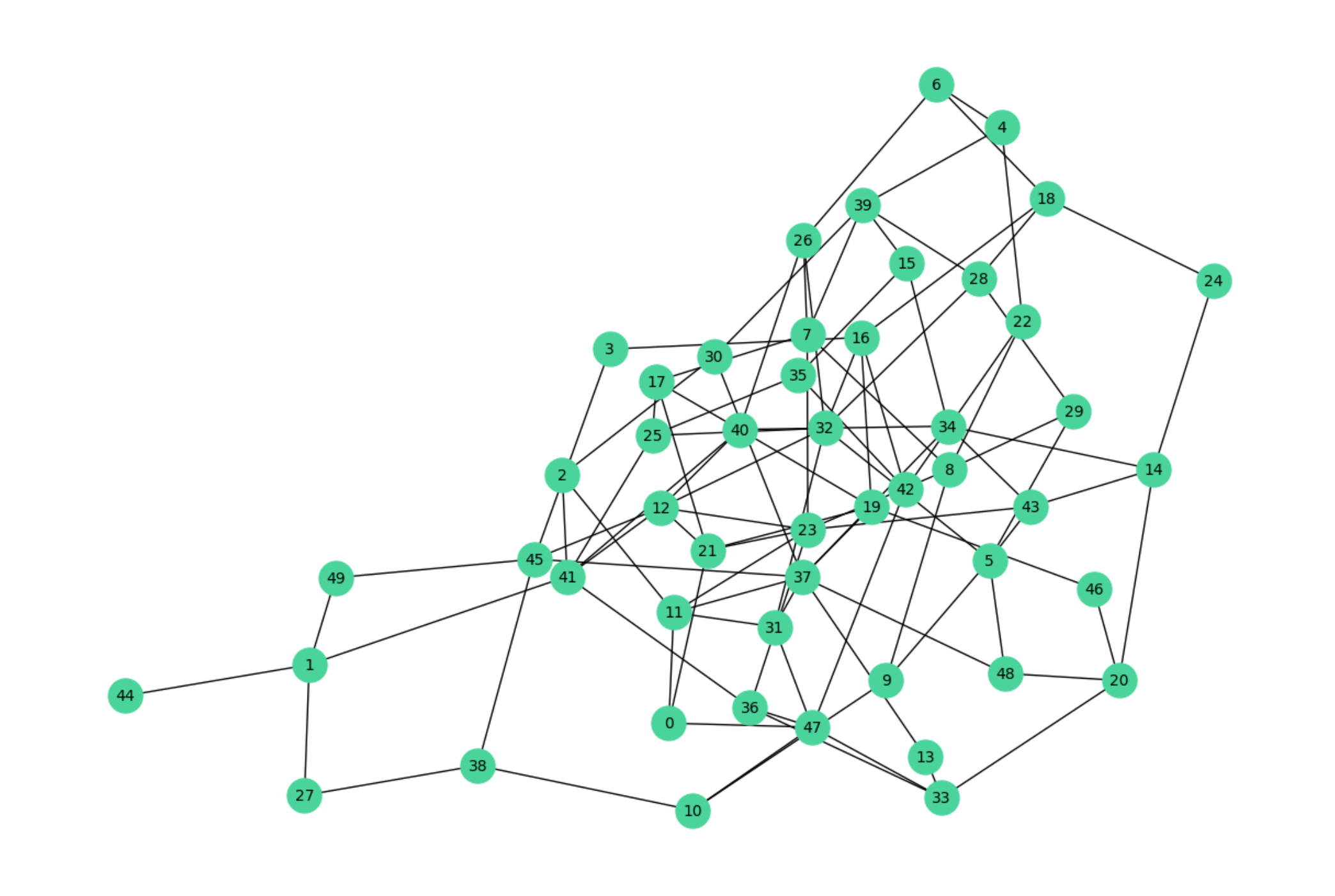
Let’s build a random graph for a given number of nodes and edges:
# build nx graph
num_nodes = 50  # variable limit of free API plan for QUBOs
num_edges = 100

nx_graph = nx.gnm_random_graph(num_nodes, num_edges, directed=False)

# visualize with pyvis
node_color = "rgb(74, 212, 156)"
edge_color = "rgb(0, 0, 0)"

# draw graph
plt.figure(figsize=(12, 8))
pos = nx.spring_layout(nx_graph)
nx.draw(nx_graph, pos, node_color="#4ad49c", edge_color="black", with_labels=True, node_size=500, font_size=10)
plt.show()
Modeling MaxCut as QUBO with Quantagonia’s API
Whether or not an edge \((i,j)\) is in the cut is expressed by
with \(x_i \in \{0,1\}\) deciding whether node \(i\) is in partition 0 or 1.
This yields the qubo
from hybridsolver.qubo import QuboModel
from hybridsolver.enums import HybridSolverOptSenses

qubo = QuboModel()

# add variables
###############
vars = {}

vars = {}
for node in nx_graph:
    vars[node] = qubo.add_variable(f"x_{node}", initial=1)

# build objective
#################
# add linear terms
for node, degree in nx_graph.degree:
    qubo.objective += degree*vars[node]
# add mixed terms
for tail, head in nx_graph.edges:
    qubo.objective -= 2 * vars[tail] * vars[head]  # asymmetric modeling, will be converted to symmetric before submitting the job
Submit the Qubo to Quantagonia’s cloud
from hybridsolver import HybridSolver, HybridSolverParameters

hybrid_solver = HybridSolver(API_KEY)

# set solver options
params = HybridSolverParameters()
params.set_time_limit(30) # setting the runtime in seconds
params.set_heuristics_only(True) # only use heuristics, change if you like to prove optimality

# solve qubo
obj_val = qubo.solve(hybrid_solver, params)
✔ Queued job with jobid 10c78c2d-00b0-4397-a4d1-5c852f3be206...
✔ Job 10c78c2d-00b0-4397-a4d1-5c852f3be206 unqueued, processing...

Quantagonia HybridSolver version 1.1.1842
Copyright (c) 2024 Quantagonia GmbH.

User-specified parameters:
Set parameter 'time_limit' to value '30.0'.
Set parameter 'heuristics_only' to value 'True'.

Read pyclient.qubo in 0.61s.
Maximize a QUBO with 50 variables and 250 nonzeros.

Presolving model. Presolved model in 0.0s.
Reduced model has 43 variables and 228 non zeros.


Running all available primal heuristics.

--------------------------------------------------------------------
  Heuristic       | Type       |      Objective Value |   Time (s) |
--------------------------------------------------------------------
  Q-MH            | classic    |           83.0000000 |       0.01 |
  Q-FV            | classic    |           83.0000000 |       0.02 |
  Q-H             | classic    |           83.0000000 |       0.02 |
--------------------------------------------------------------------

All primal heuristics finished.

Solver Results:
 - Solution Status: Feasible
 - Wall Time: 0.032 seconds
 - Objective: 83.0000000
Finished processing job 10c78c2d-00b0-4397-a4d1-5c852f3be206...
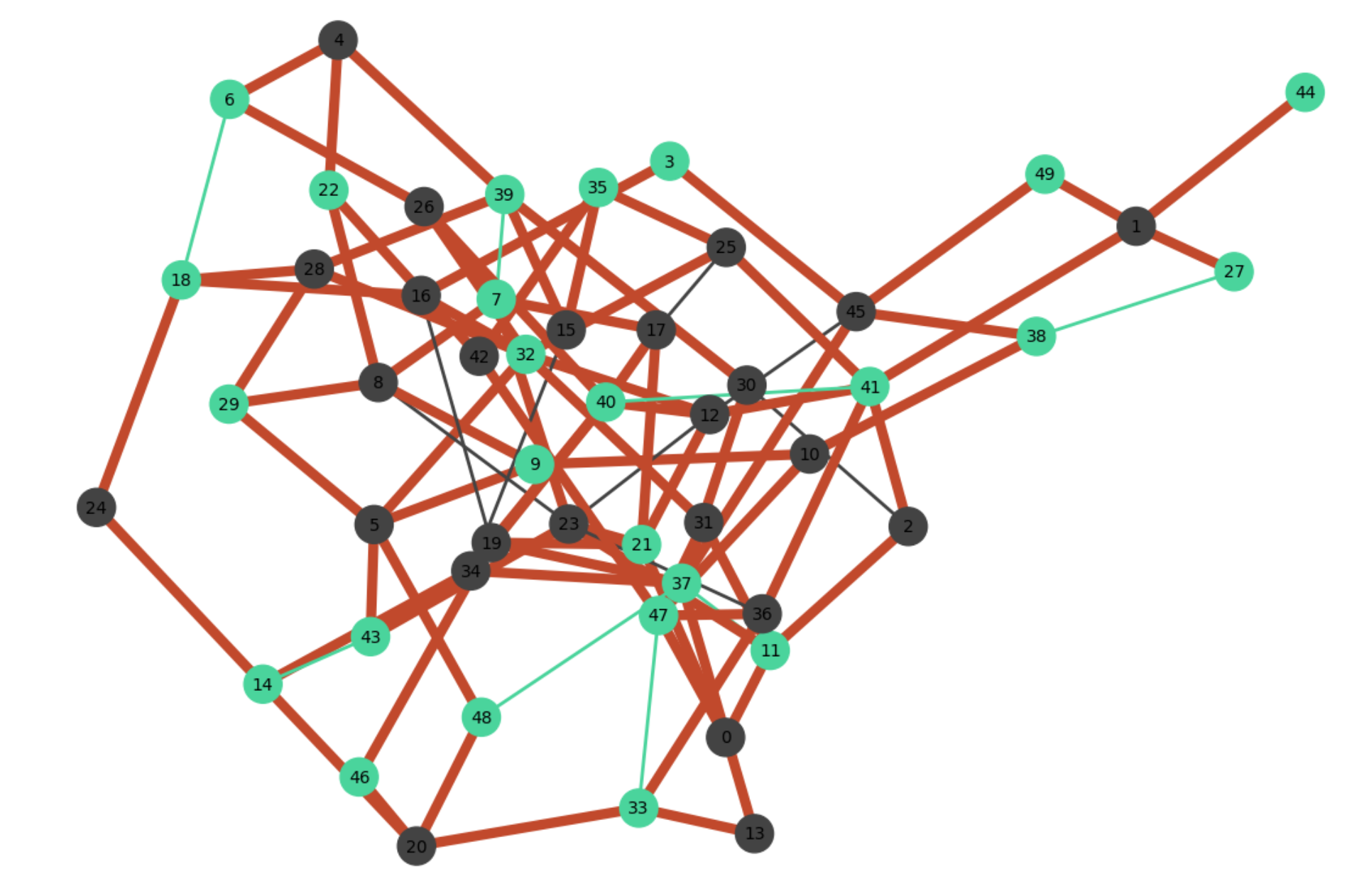
Display the solution
print(f"The proven optimal solution has {qubo.eval()} edges connecting the complementary node sets.")
The proven optimal solution has 83.0 edges connecting the complementary node sets.
# import packages
import networkx as nx
import matplotlib.pyplot as plt

# Define colors and edge widths
coloring = {0: "#4ad49c",  # quantagonia green, if node in set 0; for edges if both nodes in set 0
            1: "#c1492c",  # red, if edges are in different sets
            2: "#434343"}  # black, if node in set 1; for edges if both nodes in set 1
edge_widths = {0: 2, 1: 6, 2: 2}

# Create node and edge lists with attributes
node_colors = []
edge_colors = []
edge_width_list = []

for node in nx_graph.nodes:
    val = qubo.vars[f"x_{node}"].eval()
    node_colors.append(coloring[2 * val])

for tail, head in nx_graph.edges:
    tail_val = qubo.vars[f"x_{tail}"].eval()
    head_val = qubo.vars[f"x_{head}"].eval()
    edge_colors.append(coloring[tail_val + head_val])
    edge_width_list.append(edge_widths[tail_val + head_val])

# Draw graph
plt.figure(figsize=(12, 8))
pos = nx.spring_layout(nx_graph)
nx.draw(nx_graph, pos, node_color=node_colors, edge_color=edge_colors, width=edge_width_list, with_labels=True, node_size=500, font_size=10)
plt.show()
Need help with modeling? We are happy to coach you through your model formulation. Reach out to us at help@quantagonia.com or https://www.quantagonia.com/contact.


